Raw score distributions are fundamental tools in educational measurement that show how students performed across the full range of possible scores on an assessment.
Distribution Characteristics
Shape and Skewness
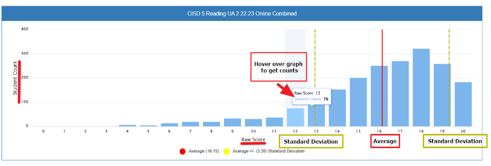
The distribution exhibits a negative (left) skew, with the majority of students scoring in the upper range (scores 13-20). The distribution shows a pronounced concentration of students achieving higher raw scores, indicating overall strong performance on this reading assessment.
Central Tendency
- Mean (Average): 16.15
- The average falls in the upper portion of the possible score range, confirming the positive performance trend
Central Tendency Calculations
Mean (x̄)
- Given: x̄ = 16.15
- Formula: x̄ = Σ(xi × fi) / N
- Where xi = raw score, fi = frequency, N = total number of students
Variability
- Standard Deviation: 3.20
- The yellow dashed lines represent the boundaries at ±1 standard deviation from the mean (approximately 12.95 to 19.35)
Standard Deviation (σ)
- Given: σ = 3.20
- Formula: σ = √[Σ(xi – x̄)² × fi / N]
Standard Deviation Boundaries
- Lower boundary: x̄ – σ = 16.15 – 3.20 = 12.95
- Upper boundary: x̄ + σ = 16.15 + 3.20 = 19.35
- Range within ±1σ: 12.95 to 19.35 (marked by yellow dashed lines)
Score Distribution Patterns
- Low Scores (0-6): Minimal student representation, with very few students scoring in this range
- Mid-Range (7-12): Gradual increase in frequency, with the tooltip indicating 20 students scored a 7
- High Scores (13-20): Highest concentration of students, with peak frequencies occurring around scores 17-18 (approximately 300+ students)
- Maximum Frequency: Appears to occur at raw score 18, with over 300 students
Statistical Boundaries
The vertical dashed lines (yellow) mark the standard deviation boundaries, helping identify students who fall outside the typical performance range for intervention or advanced instruction consideration.
This distribution pattern suggests the assessment was appropriately calibrated for the student population, with most students demonstrating proficiency while still providing differentiation across the score range.
Score Range Analysis
- Theoretical Range: 0-20 (21 points)
- Actual Range: Approximately 4-20 (16 points observed)
- Range Utilization: 16/21 = 76.19% of possible scores
Performance Categories
- Below Average (< 12.95): z < -1.0, approximately 16% of students
- Average Range (12.95-19.35): -1.0 ≤ z ≤ +1.0, approximately 68% of students
- Above Average (> 19.35): z > +1.0, approximately 16% of students
Z-Score Calculations (standardized scores)
Formula: z = (x – x̄) / σ = (x – 16.15) / 3.20
Examples:
- Score of 20: z = (20 – 16.15) / 3.20 = +1.20
- Score of 13: z = (13 – 16.15) / 3.20 = -0.98
- Score of 7: z = (7 – 16.15) / 3.20 = -2.86
Percentile Estimations
Based on normal distribution approximation:
- Score of 13 (z ≈ -1.0) ≈ 16th percentile
- Score of 16.15 (mean) = 50th percentile
- Score of 19.35 (+1σ) ≈ 84th percentile
Skewness Indicator
The visual distribution suggests negative skew, where:
- Mean (16.15) < Mode (appears to be around 17-18)
- Tail extends toward lower scores
- Estimated skewness coefficient likely between -0.5 to -1.0